Demystifying Deep Learning: Part 2

Linear and Logistic Regression

Introduction:

Today, we get our hands dirty with our first machine learning algorithms! Whilst we are starting out simple, these algorithms are still very useful and can be used as a baseline to measure the later machine learning algorithms we cover - to ensure the algorithm is behaving as we expect.

Intuition:

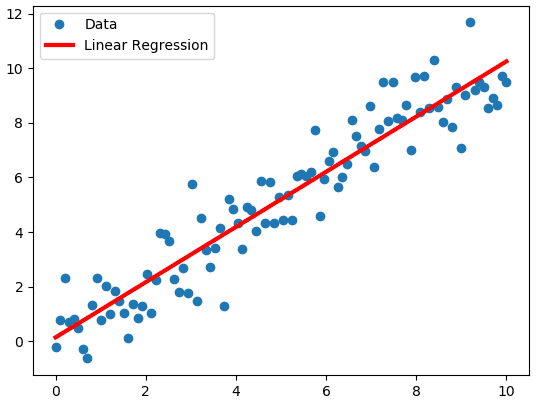
Often when we have a set of data points in science, we want to draw a straight line of best fit through the points (see picture above). Linear Regression involves learning this straight line of best fit, only with more dimensions - instead of axes $x$ and $y$ , we have axes $x_1, x_2, ... ,x_n$ and $y$.

In Linear Regression, we use this straight line of best fit and the values for $x_1, x_2, ... ,x_n$ , which we call input features to predict the value of the output $y$. This is useful in regression tasks, e.g. housing prices.

Now instead of a real number output, suppose we wanted to classify this input as one of two classes e.g. fraudulent vs non-fraudulent credit card data. Logistic Regression involves taking this output and applying a decision function to this - we end up with a probability - if close to 1 the input is one class, and if closer to 0 the input is the other class. We can think of this probability as the “confidence” the algorithm has.

Side note: The name logistic regression is a little confusing as it is a classification algorithm, however this is because the term regression in the context of machine learning differs from regression in statistical maths. For our purposes, we’ll use the definition in the first blog post of the series - of real-valued output.

Maths:

The equation for linear regression extends naturally from the equation of a straight line:

$y= mx + c$

Just like how $m$ is the gradient of the line, we assign weights to the input features - let $w_i$ denote the weight corresponding to feature $x_i$ - you can loosely think of $w_i$ as the gradient of the line in the direction of the $x_i$ axis.

Another way of thinking of fitting a line of best fit is as projecting the original data points $y$ onto the line, denoting our projection as $\hat{y}$ . Extending this to $n$ dimensions, instead of a line we consider a n-dimensional hyperplane that we are projecting our data points onto.

So the equation for linear regression is:

$\hat{y} = \sum_{j=1}^{n}{w_jx_j} + b$

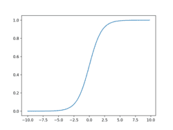
For logistic regression, we apply the sigmoid function $\sigma(x)$ to this output - this scales the values to between 0 and 1 (to get the probability) - see the graph below:

$\sigma(x) = \frac{1}{1+e^{-x}}$

$\hat{y} = \sigma(\sum\_{j=1}^{n}{w_jx_j} + b)$

Notation:

One convention we will follow is $(x^{(i)}, y^{(i)})$ refers to the $i^{th}$ training example, with $\hat{y}^{(i)}$ the corresponding prediction by the model. In general $^{(i)}$ refers to the value for $i^{th}$ training example. We use $m$ to denote the number of examples in the training set and $n$ to denote the number of input features.

Matrices

We will also represent our operations as matrix multiplications, since it is cleaner to express and also more efficient when implemented compared to a for loop across the values.

So here, we store our input in a n x m matrix $X$ and the labels as a 1 x m matrix $Y$ . Then we can represent $W$ as a 1 x n matrix and express the calculation as:

$\hat{Y} = W.X + b$ - note $\hat{Y}$ has same dimensions as labels $Y$.

In general, if we have an equation of form $C_{ij} = \sum_k A_{ik} B_{kj}$ this corresponds to a matrix multiplication $C = A.B$

(Here we have $\hat{Y}_{1i} = \sum_{j=1}^{n}{W*{1j}X*{ji}}$)

Code:

We will be writing the code snippets in Python and we are using Numpy (a linear algebra library) to carry out the maths operations.

Our motivating problem for linear regression is the Boston Housing Prices dataset, and for logistic regression the Breast Cancer dataset (classifying tumour as benign/malignant). See the Jupyter notebook to see the input preprocessing.

The intention of the blog posts is to highlight the pertinent parts of the code - the notebook accompanying the blog post can be used to view the rest of the code and implement the algorithm on a concrete problem to consolidate.

With all that said, let’s dive into the code - note how np.dot is used for matrix multiplication.

import numpy as np #we use numpy to do the maths operations

#_lin refers to linear regression, _log for logistic regression
#similarly _train for training set, _test for test set.

#initialise weights and bias to random values
# we'll get to training them  in the next blog post.
W_lin = np.random.randn(Y_lin_train.shape[0], X_lin_train.shape[0]) #1xm matrix
b_lin = np.random.randn(Y_lin_train.shape[0],1) #1x1 matrix

W_log = np.random.randn(Y_log_train.shape[0], X_log_train.shape[0])#1xm matrix
b_log = np.random.randn(Y_log_train.shape[0],1)) #1x1 matrix

#Linear Regression
def forward_lin(X, W, b):
    return np.dot(W,X)+b

def sigmoid(z):
    return 1.0/(1+np.exp(-z))

#Logistic regression
def forward_log(X,W,b):
    return sigmoid(forward_lin(X,W,b))

Conclusion:

At this point, you’re probably thinking, “Great! But this is just maths, where is the learning?“. Hold tight, because in the next blog post we’ll be doing just that! We will look at how exactly most machine learning algorithms even “learn”, and how we evaluate their performance.