Privacy Preserving Machine Learning: Part 1

Deep Learning with Differential Privacy (DP-SGD Explained)

Last updated: December 26, 2021

Many of the world’s greatest machine learning problems require access to sensitive data, such as patient records for cancer detection. The issue is that machine learning models have a tendency to memorise private data, even if they aren’t overfitting

How can we train our models whilst still preserving privacy?

Through a technique called differential privacy.

In this post I’ll explain what differential privacy is, and go through the seminal differentially-private machine learning algorithm: DP-SGD (differentially-private stochastic gradient descent).

Why not just anonymise the data?

Wait wait, why do we need a special privacy-preserving algorithm at all? Surely the easiest solution is to just remove any private information by anonymising the data?

Well, that doesn’t work.

Netflix anonymised the training set for its recommender challenge by replacing all names with random ids. Turns out that by linking this dataset with public IMDB review ratings, researchers were able to deanonymise people.

Likewise, Strava got into hot water when it released an anonymised aggregate heatmap of location data, as it inadvertently revealed the location of military bases.

Every time we perform any form of statistical analysis, we leak a little information about the data.

See, if I tell you that the mean of the ages of the participants of a dataset is 34, then I’ve revealed a bit of information about the participants.

If we want total privacy, we learn nothing about the data.

Revealing the mean age tells us less than revealing all of the participants’ ages. But that’s a bit wishy-washy: let’s quantify this loss of privacy.

Enter Differential Privacy

Differential privacy lets us quantify the “privacy” of any mechanism $M$ that interacts with data $D$ to produce some output.

The definition of a mechanism is intentionally broad, it covers everything from statistical analysis through database queries to even simple pen & paper calculations.

M: Data -> Output

In the case of machine learning, the mechanism $M$ isn’t just the final model, it’s the entire process of training a model on the dataset $D$ and using that model’s predictions.

Let’s use an example to illustrate the goal of differential privacy.

Example: training on a cancer dataset.

Say we’re training a model on a cancer dataset $D$, and we ask it to predict if a particular patient Bob has cancer. We’ll call this entire mechanism (training a model and then predicting whether Bob has cancer) $M$.

$P(M(D)=\text{“Bob has cancer”}) = 0.55$

If we train a model on the same dataset augmented with Bob’s records and it improves from 55% to 57% confident,

$P(M(D+\text{Bob})=\text{“Bob has cancer”}) = 0.57$

then maybe Bob’s data says he has cancer, but maybe it’s just that the model got more confident overall with more data. Bob’s privacy comes from this plausible deniability of him having cancer.

What if it actually became 80% confident Bob has cancer?

$P(M(D+\text{Bob})=\text{“Bob has cancer”}) = 0.80$

Just by adding Bob to the dataset, the outcome “Bob has cancer” has become significantly more likely, so it’s pretty clear that Bob does in fact have cancer, and the mechanism $M$ leaked information about Bob!

We can quantify the privacy loss as the log of the ratio of the probabilities before and after Bob was added to the dataset: i.e.

$\Large{\log{\frac{P(M(D+\text{Bob}))=\text{“Bob has cancer”})}{P(M(D)=\text{“Bob has cancer”})}}}$.

So if we plug in the numbers for our two examples, we have:

$\large{\log{\frac{0.57}{0.55}} = 0.0357}$

$\large{\log{\frac{0.80}{0.55}} = 0.375}$

We can quantifiably say that the second outcome has 10x the privacy loss.

The key idea behind differential privacy is to limit this difference in performance: the model should make a make a similar inference about me whether or not I individually opt-in to the dataset, thus preserving my privacy.

In the equations that follow that formally define differential privacy, we look at datasets $D$ and $D'$ that differ in one data record (i.e. we add/remove a record). We consider the privacy loss on a set of outcomes $S$:

$\Large{\log{\frac{P(M(D) \in S)}{P(M(D') \in S)}}}$.

Mathematical definitions of differential privacy

If we had zero privacy loss, then from our definition the probabilities $P(M(D) \in S)$ and $P(M(D') \in S)$ would be the same → we wouldn’t have learnt anything from that record we added/removed.

So we have to be a bit more flexible and specify an upper-bound on our privacy loss, which we denote with an $\epsilon$. We call this our privacy budget.

$\Large{\log{\frac{P(M(D) \in S)}{P(M(D') \in S)}} \leq \epsilon}$.

We tune this $\epsilon$ to trade-off how much we learn vs the privacy of the individual.

$\epsilon$-Differential Privacy

We can rearrange this inequality to get our first mathematical definition of privacy.

$\large{{P(M(D) \in S)} \leq e^\epsilon {P(M(D') \in S)}}$.

So if we can bound this privacy loss by $\epsilon$ for any datasets D and D’ whatever the outcome we observe, we have a formal guarantee of privacy. We say the mechanism $M$ is $\epsilon$-differentially private.

($\epsilon$-$\delta$)-Differential Privacy

This bound is very tight - in practice we allow for a tiny failure probability $\delta$ (much less than the probability of a given individual).

$\large{{P(M(D) \in S)} \leq e^\epsilon {P(M(D') \in S)}} + \delta$.

We say the mechanism $M$ is ($\epsilon$-$\delta$)-differentially private.

Privacy is no longer subjective

I want to just take a moment to pause here and appreciate how elegant this solution is:

• Privacy isn’t subjective - we can quantitatively compare mechanisms by comparing their privacy budgets.
• This privacy guarantee is rock solid - the bound holds no matter how the attackers try to post-process the outputs of the mechanism or combine them with other data.

How do we achieve this guarantee?

So differential privacy gives us this definition, but how do we achieve it in practice?

Adding noise

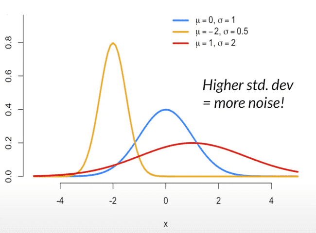
We can limit the privacy loss by adding noise. Think of an image: the more noise you add, the fuzzier the image, so the less you learn from it.

Every time you add a bit of random noise, you spread the range of possible values the input could have been. So if I take my age as 35, and then add noise sampled from a Gaussian distribution with a standard deviation of 5 - then within a 95% confidence interval my age could be anywhere between 25 and 45.

The noise essentially smooths the probabilities and prevents one outcome from becoming much more likely. The smaller your privacy budget, the more noise you need to add.

Subsample and aggregate

There’s another technique we can use add “randomness’ - sampling. If we have a large dataset, and we sample a random fraction $q$ rather than the entire data, then the privacy amplification theorem states that our privacy budget needed reduces by a factor of $q$.

I.e. a ($\epsilon$-$\delta$)-differentially private mechanism M becomes ($q\epsilon$-$q\delta$)-differentially private

Composition of privacy budgets

Now if you’ve ever played the game 20 questions, you know you can hone in on the answer by asking enough questions. (This is the Fundamental Law of Information Recovery.)

So the more queries we have, the larger the privacy loss.

Luckily for us, this is easy to compute: we can add up our privacy budgets:

If we have a mechanism $M_1$ that has a budget of $\epsilon_1$, and another mechanism $M_2$ that has budget $\epsilon_2$ , the overall budget we need is at most $\epsilon_1$ + $\epsilon_2$.

And it turns out this also follows for ($\epsilon$-$\delta$)-differential privacy, i.e. the overall mechanism ($M_1$ followed by $M_2$) is $(\epsilon_1 + \epsilon_2)$-$(\delta_1+\delta_2)$-differentially private.

This budget is a loose upper bound and with careful analysis we can prove tighter bounds. But more on that in a second! Let’s apply what we’ve learnt so far to our deep learning models.

DP-SGD (Deep Learning with Differential Privacy)

Now we have the building blocks in place, we can tackle the seminal paper that applies differential privacy to deep learning models.

This paper proposes a modification to stochastic gradient descent algorithm to make it differentially-private: i.e. differentially-private stochastic gradient descent or DP-SGD for short.

The DP-SGD Algorithm

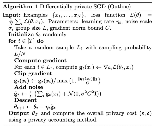
The aim of the algorithm is to limit the privacy loss per gradient update, by post-processing the gradient update in 2 steps:

1. We clip the gradients - scaling the gradient so it has a max L2 norm of $C$. Clipping the gradient bounds the amount of information in a given update, which lets us reason about the maximum privacy loss.

2. We then add noise proportional to our clipping norm $C$ to the gradient updates. You can see we sample from a normal (Gaussian) distribution with standard deviation $C\sigma$. We call $\sigma$ the noise multiplier.

These hyperparameters $C$ and $\sigma$ can be tuned to get a particular ($\epsilon$-$\delta$) guarantee for each individual step of training.

The specific value of $C$ doesn’t actually affect the ($\epsilon$-$\delta$) guarantee, since a larger value of $C$ means more noise will be added to compensate.

It’s possible to show that $\sigma = \sqrt{2 \log{\frac{1.25}{\delta}}} / \epsilon$ gives us the ($\epsilon$-$\delta$) guarantee for that individual step of gradient descent. For brevity, we’ll skip the mathematical derivation in this blog post.

So now we have an ($\epsilon$-$\delta$) guarantee for an individual step of gradient descent, how do we compute the privacy guarantee of the overall training process?

Moments accountant

This leads us to the second key contribution of this paper: the privacy analysis through a technique called the moments accountant.

The maths for the moments accountant technique is rather heavy, so I’ll have a follow-up blog post dedicated to it, but in this post I want to demonstrate its benefits.

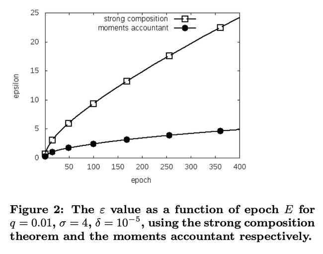
Getting a tighter bound on the privacy budget means we can run our training process for longer given the same privacy budget.

Let’s look at a simple privacy analysis based on the techniques we’ve looked at so far:

If each step has a ($\epsilon$-$\delta$) guarantee, then:

• Sampling minibatch with some probability $q = \frac{L}{N}$, gives us a revised guarantee of ($q\epsilon$-$q\delta$)

• Adding up the $T$ steps of gradient descent gives us an overall ($qT\epsilon$-$qT\delta$) differential privacy guarantee

So you can see our budget scales with the number of steps $T$.

Prior to this paper, the tightest bound came from the strong composition theorem, which gave a bound of ($O(q\epsilon \sqrt{ T \log{\frac{1}{\delta}}} )$, $Tq\delta$) differential privacy.

The moment accountant gets us an even tighter bound: the overall training process is ($O(q\epsilon \sqrt{ T} )$, $\delta$)-differentially private.

See that’s two major improvements:

• First the budget is now proportional to $\sqrt{T}$ not $T$, so you can run the algorithm for longer
• Secondly the failure probability is $\delta$ (not $Tq\delta$), so it is independent of the number of training steps $T$.

Implementing DP-SGD

DP-SGD is implemented as part of the TensorFlow Privacy library. Pytorch also has an equivalent library for differential privacy called Opacus.

This makes using differential privacy as simple as just swapping out your optimiser.

from tensorflow_privacy.privacy.optimizers import dp_optimizer

# replace this
  optimizer = tf.train.GradientDescentOptimizer(
          learning_rate=__)

# with this
 optimizer = dp_optimizer.DPGradientDescentGaussianOptimizer(
          l2_norm_clip=__,
          noise_multiplier=__,
          num_microbatches=__,
          learning_rate=__)

Rounding off this blog post with some practical notes:

• We don’t need to do learning rate decay, as DP-SGD never gets to a regime where we’d converge (because of the noise).

• The size of your minibatch affects privacy - larger batches mean less noisy training but less privacy, as we’re sampling a larger fraction of the data (remember $q=\frac{L}{N}$).

• Rather than clipping each gradient separately, Tensorflow specifies microbatches of gradients to average the norm over, for performance reasons.

• In practice DP-SGD tends to only work well for larger datasets, as the larger the dataset the less noise you need to achieve a given privacy budget.